Live Trade Sequence Replayed Across Six Capital Levels.
Three Cost Models Applied. Slippage Drawn From 4,957 Actual Broker Fills.
Under zero friction, linear drag, and a nonlinear power-law stress model — from $1M to $50M. The edge does not disappear at institutional scale.
The Capacity Model, Explained
In Under Six Minutes.
We Did Not Model Blind.
We Pulled 4,957 Actual Fills.
Before scaling a single trade, we went into the IC Markets EU execution log and extracted every take-profit fill from the live record. Exit fill price against requested take-profit price, divided by mid, multiplied by ten thousand. That is the slippage in basis points for every exit. These figures — not industry assumptions — became the calibration anchor for both cost scenarios.
How Is Slippage Modelled — And How Conservative Is It?
The strategy exits exclusively on limit orders — take-profit targets placed at the time of entry. Limit order exits do not push price. They do not manufacture their own slippage. This property holds at $30M and remains true at $100M in trillion-dollar daily turnover markets. The execution log is the proof. Limit orders are also unaffected by spread widening — they wait for their price.
The slippage calibration is drawn from executed limit fills and therefore bounds fill-quality degradation — not fill-probability degradation. What is measured is how much worse the fill price was than requested, on fills that occurred. What it does not capture is the risk that limit orders go unfilled entirely at scale. In trillion-dollar daily FX turnover, fill-probability degradation at $30M peak notional of ~$900k per position is not a material concern — but the distinction is disclosed.
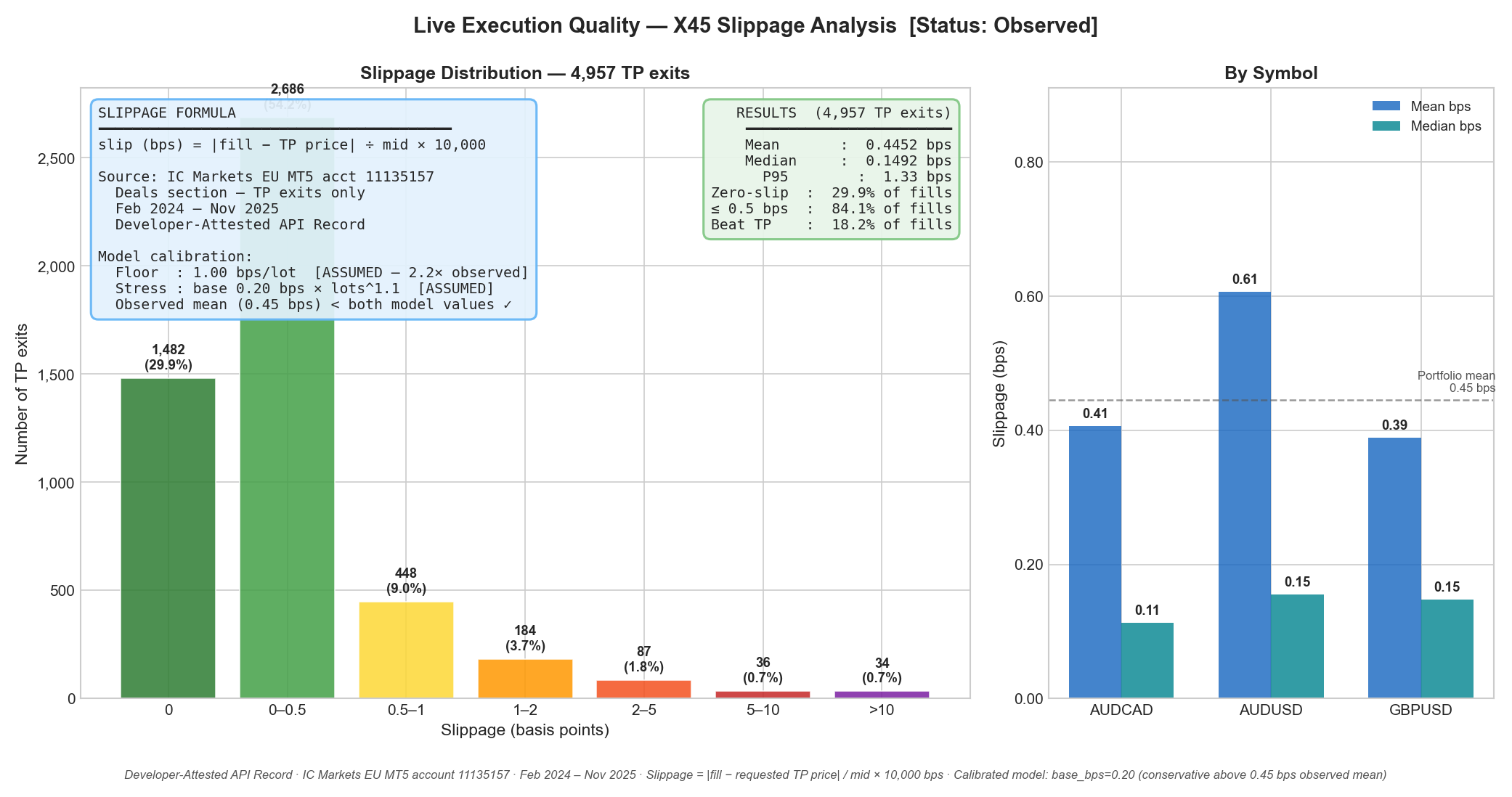
Each section below poses the question, presents the calculation, and states the answer directly. All figures are derived from the same 4,999-trade live record. No backtest. No simulation.
Three Scenarios. Built To Break
The Thesis If It Can Be Broken.
Every trade in the live record was scaled proportionally across six capital levels. Real commissions and swap costs from the broker log were applied at scale. Slippage was modelled three ways — one conservative, one deliberately punishing, one optimistic ceiling. CAGR is annualised across 19 active trading months. The honest calculation.
How Is The Strategy Actually Deployed At Scale — And How Does The Stress Test Differ?
The capacity analysis runs two methodologies in parallel. Understanding the distinction is essential to interpreting the CAGR outputs correctly.
Every live trade is replayed with lot sizes scaled proportionally to capital — no position cap applied. This deliberately produces oversized positions at large AUM levels.
Purpose: Stress test. Does the underlying alpha survive uncapped proportional scaling? If it does, it trivially survives operational deployment — because capped positions are smaller, not larger.
The 3% per-position cap is enforced. At $30M, this limits peak notional per trade to ~$900k — a level architecturally invisible in BIS-verified FX daily volume.
Purpose: Real deployment constraint. The 3% cap means actual traded positions are smaller than Test A — making Test A the conservative, harder case. Both are shown; Test A is the binding stress test.
Q2 answered: The stress test (Test A) applies uncapped proportional scaling — deliberately oversized positions that the 3% operational cap would prevent. Test B is the real deployment model: peak notional ~$900k per trade at $30M, architecturally invisible in BIS-verified FX volume. Test A is the harder case. If the edge holds there, it holds in operational deployment.
Net annualised return across six capital levels under each cost model. Denominator: 19 active trading months. All figures derived from the same 4,999-trade live record scaled proportionally. Linear CAGR is flat across all levels — proportional drag means proportional cost, so the annualised rate is invariant to capital. Nonlinear crosses linear at ~$24M where power-law compounds faster.
| Capital Level | Zero Friction | Floor Case (Linear) | Stress-Tested (Nonlinear) | Spread (Best–Worst) |
|---|---|---|---|---|
| $1M | 35.5% | 29.3% | 32.2% | 6.2pp |
| $5M | 35.5% | 29.3% | 31.0% | 6.2pp |
| $10M | 35.5% | 29.3% | 30.3% | 6.2pp |
| $20M | 35.5% | 29.3% | 29.5% | 6.2pp |
| $30M | 35.5% | 29.3% | 29.0% | 6.5pp |
| $50M | 35.5% | 29.3% | 28.3% | 7.2pp |
The linear floor holds flat at 29.3% across all capital levels — proportional scaling means proportional cost, so the annualised rate is capital-invariant. The nonlinear model starts above the linear floor at small scale but crosses it at approximately $24M AUM, where the power-law exponent causes drag to compound faster than capital growth. At $30M: nonlinear generates $3.7M of additional drag versus $3.5M linear. The stress floor is the harder test above $24M. The thesis holds under both. At $30M, X45 tolerates approximately 4 basis points of all-in drag before the economics break.
The nonlinear effective rate grows with capital multiplier M = C / $7,700. Formula: eff_bps = 0.20 × M0.2. Below ~$24M the nonlinear model is cheaper than linear. Above it the power-law bites harder — making it the genuine stress floor at institutional scale.
Crossover: 0.20 × M0.2 = 1.00 → M = 55 = 3,125 → C* = 3,125 × $7,700 = $24.06M
| Capital | Multiplier (M) | NL eff_bps | Linear drag | NL drag | NL vs Linear |
|---|---|---|---|---|---|
| $1M | 129.9× | 0.529 bps | $0.12M | $0.06M | NL cheaper |
| $5M | 649.4× | 0.730 bps | $0.58M | $0.43M | NL cheaper |
| $10M | 1,298.7× | 0.839 bps | $1.17M | $0.98M | NL cheaper |
| $20M | 2,597.4× | 0.964 bps | $2.34M | $2.25M | NL cheaper |
| $30M | 3,896.1× | 1.045 bps | $3.50M | $3.66M | NL = stress floor |
| $50M | 6,493.5× | 1.158 bps | $5.84M | $6.76M | NL = stress floor |
All drag figures from live engine. Base NAV $7,700. X45 Capacity Engine · stress exponent α=1.2 (recalibrated Sep 2026, Jawad review). $30M row = proposed capital level only — not a confirmed safe figure.
Why This Cost Model — And What Changes If The Exponent Assumption Is Wrong?
The nonlinear exponent is not an empirical finding — it is a deliberate stress-test specification. Here is the provenance, and a sensitivity sweep to show the conclusion is not dependent on the 1.2 choice.
The X45 Capacity Engine (recalibrated Sep 2026, Jawad Howard methodology review) uses a nonlinear power-law cost model: slippage ∝ lotsα, with the effective rate per unit given by eff_bps = 0.20 × Mα−1. The stress exponent α = 1.2 is a formula parameter — it is not a version label for the engine. Its purpose is to produce a scenario that is genuinely more punishing than linear drag above $24M. Exponent α = 1.1 failed that test; α = 1.2 passes it.
Empirical baseline: 0.45 bps mean observed slippage (4,957 TP fills) — this is what the broker actually recorded. Conservative floor: 1.00 bps linear (proportional, capital-invariant). Stress model: eff_bps = 0.20 × M0.2 — super-linear above $24M (where M = C/$7,700, and the exponent on M is α−1 = 0.2).
| Stress Exponent | $10M | $30M | $50M | Note |
|---|---|---|---|---|
| 1.1 | 30.5% | 29.2% | 28.7% | NL cheaper than linear at $30M — not a valid stress case |
| 1.2 (base) | 30.3% | 29.0% | 28.3% | Genuine stress floor — NL exceeds linear above $24M |
| 1.3 | 30.1% | 28.7% | 27.7% | More punishing — conclusion unchanged |
The conclusion — that the edge survives at institutional scale — holds across all three exponent variants. The 1.2 base case is neither the most aggressive nor the least. It is calibrated to be the valid stress case.
Q3 answered: The 1.2 exponent is the HavenAlgo capacity calculator specification — not a retrospective choice. The sensitivity sweep shows that at 1.1 the nonlinear scenario is cheaper than linear (not a valid stress case), while at 1.2 and 1.3 the conclusion — edge survives at $30M — is unchanged. The analysis is not dependent on the specific exponent.
The proportional scaling model intentionally produces positions that exceed the 3% per-position operational cap at large capital levels. That is by design. Proportional scaling is the most punishing capacity stress test the live record can generate: every trade is replicated at full scale with no operational modification applied.
If the edge survives this test, it survives deployment constrained by the 3% cap — because operationally capped positions are smaller than what is modelled, and therefore cheaper to execute. The model is more conservative than actual deployment, not less.
The 3% cap is an operational deployment control that governs how the strategy would be run at size. The stress test answers a different question: does the alpha degrade under proportional scale? These are separate constructs with separate purposes. The model answers the former. The cap governs the latter. Conflating them understates the conservatism of the analysis.
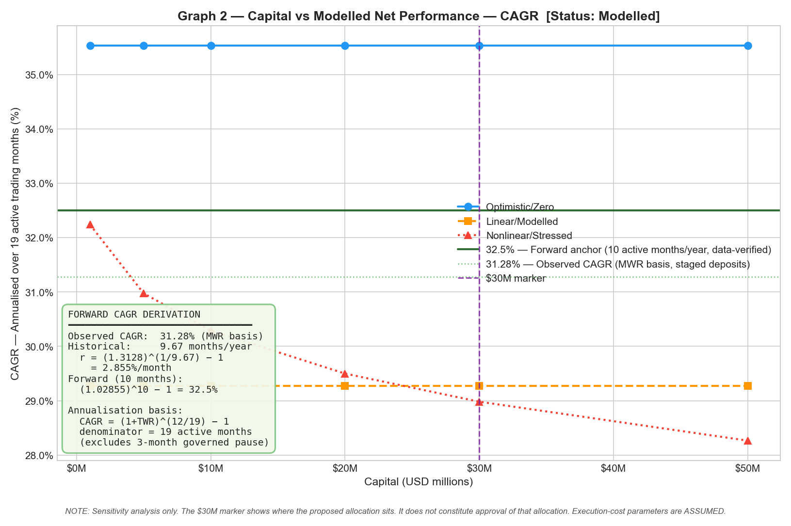
Where Does The Nonlinear Model Cross The Linear Floor — And Why Does The Crossover Point Matter?
The point at which increasing capital begins to degrade the CAGR curve — plotted across all three cost scenarios from $1M to $50M. The frontier shows where, and by how much, the edge compresses. Zero friction is flat. Linear is flat. Nonlinear curves downward — the power-law compounds. The crossover at ~$24M is where nonlinear becomes the binding constraint.
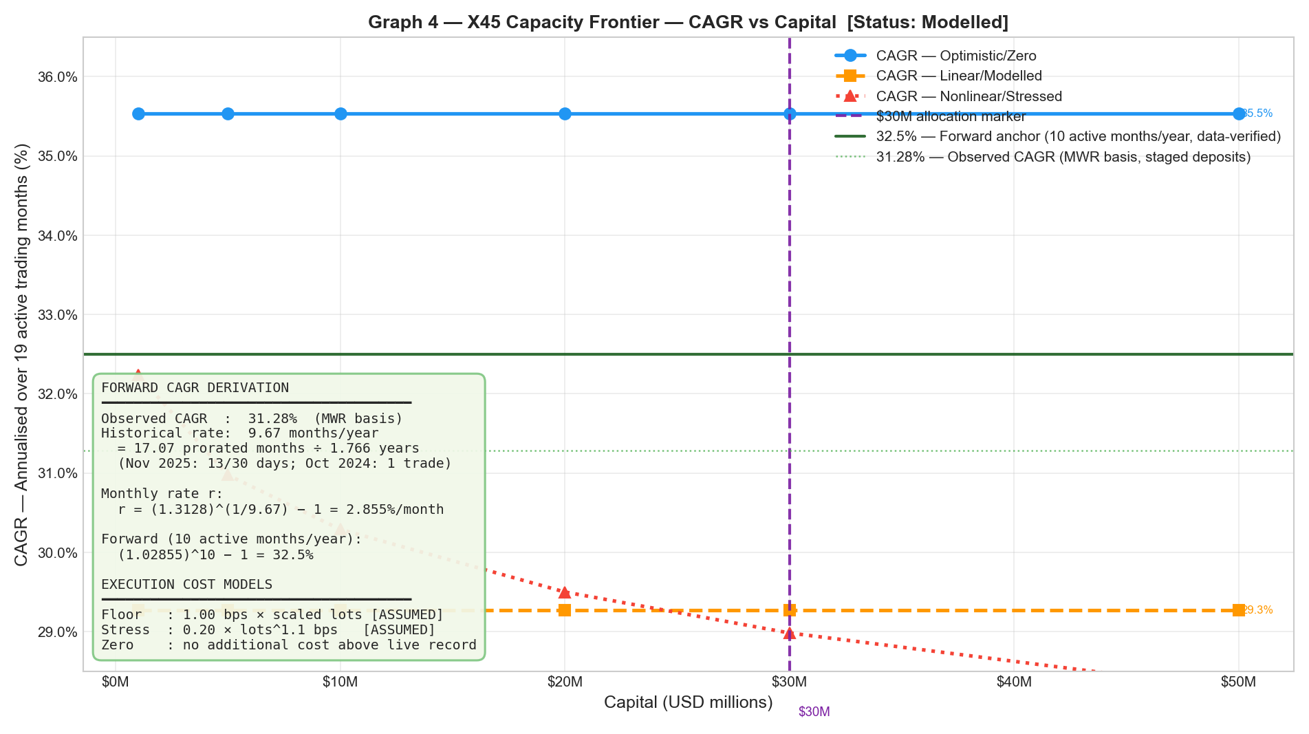
Q1 answered: Yes. The edge survives proportional scaling across all six capital levels tested ($1M–$50M) under all three cost scenarios. The nonlinear stress CAGR at $30M is 29.0% — only 0.3pp below the linear floor. The alpha does not degrade materially at the proposed campus tranche allocation level.
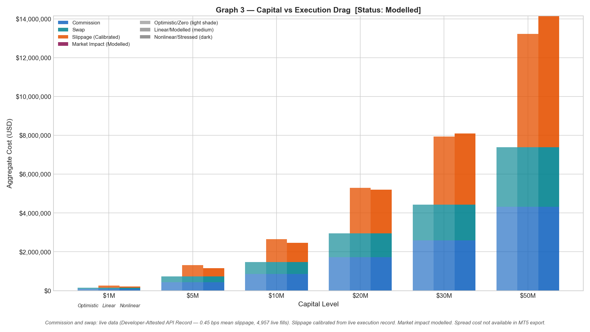
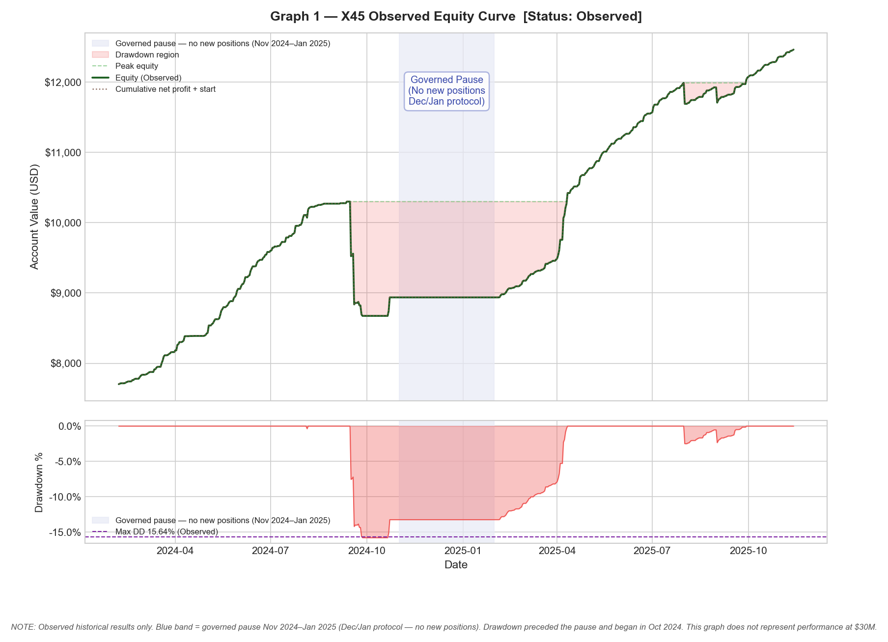
The Capacity Test Confirms What
The Architecture Already Implied.
These are not incidental properties. The algorithm was built on structural characteristics that are scale-invariant by design. Each is verifiable from the live execution record.
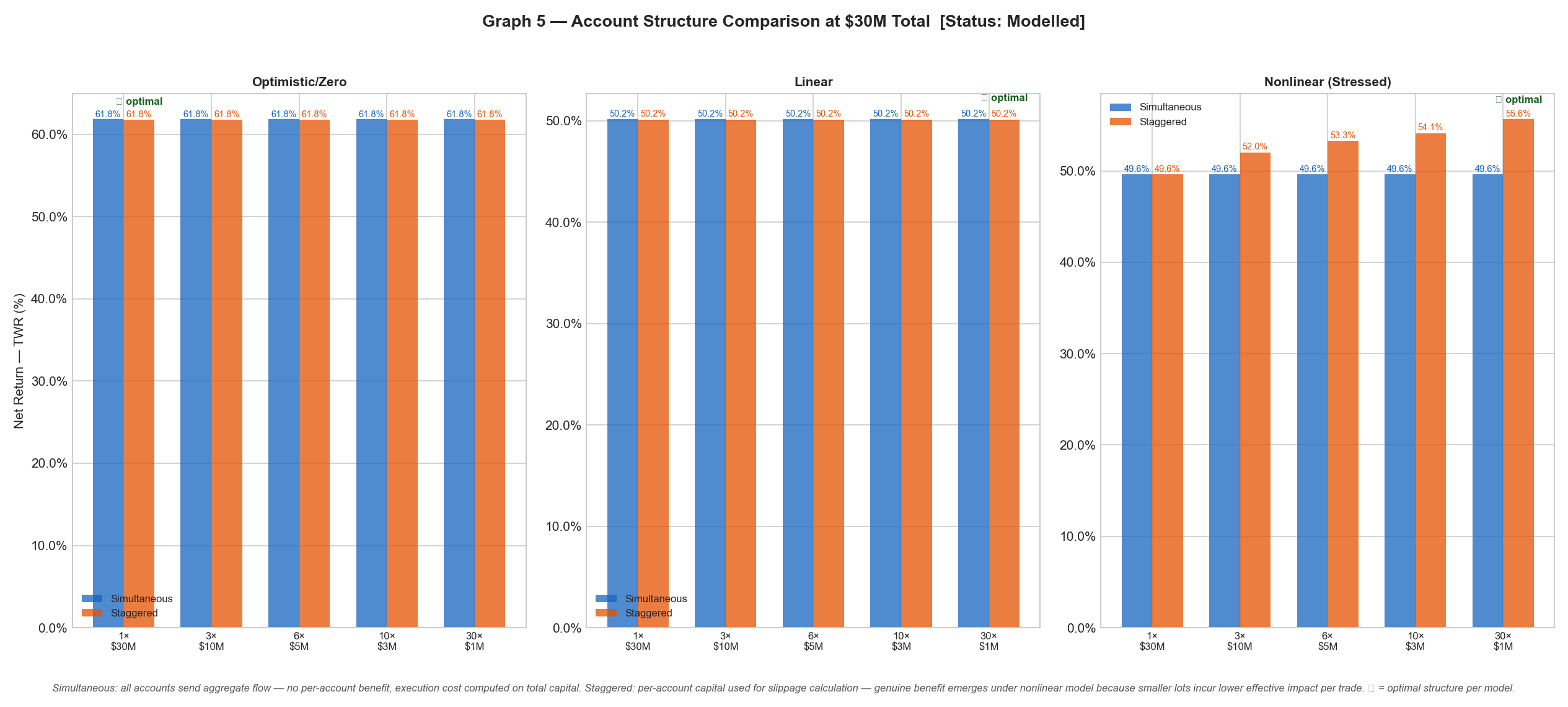
Does Splitting Capital Across Multiple Accounts Reduce Execution Cost Drag?
Under a nonlinear power-law model, account fragmentation reduces aggregate drag — because each account's capital multiplier is smaller. The calculations below use the X45 Capacity Engine with stress exponent α = 1.2 for $30M split across different numbers of accounts.
Under a nonlinear power-law model, splitting the same total capital across multiple accounts reduces aggregate drag — because each account's multiplier M = Cper/$7,700 is smaller, pulling the effective rate back down the power curve. Splitting across ≥2 accounts eliminates the nonlinear cost penalty entirely. At 2+ accounts, the nonlinear stress CAGR exceeds the linear floor (29.3%).
| N Accounts | AUM / Account | M per Account | eff bps (NL) | Total Drag | NL CAGR | vs Linear Floor |
|---|---|---|---|---|---|---|
| 1 (single) | $30M | 3,896× | 1.045 bps | $3.66M | 29.0% | −0.3pp |
| 2 | $15M | 1,948× | 0.910 bps | $3.19M | 29.9% | +0.6pp |
| 3 | $10M | 1,299× | 0.839 bps | $2.94M | 30.3% | +1.0pp |
| 5 | $6M | 779× | 0.758 bps | $2.65M | 30.8% | +1.5pp |
| 10 | $3M | 390× | 0.660 bps | $2.31M | 31.4% | +2.1pp |
| 30 | $1M | 130× | 0.529 bps | $1.85M | 32.2% | +2.9pp |
Total drag at N accounts = single-account drag ÷ N0.2. Formula: 0.20 × (Mtotal/N)1.2 × N = 0.20 × Mtotal1.2 / N0.2. Linear floor CAGR (29.3%) shown for reference — fixed regardless of fragmentation. Multi-account MAM/PAMM structure supports this architecture natively.
Q4 answered: Yes, materially. At just 2 accounts the nonlinear stress CAGR (29.9%) exceeds the linear floor (29.3%) — the nonlinear cost penalty is eliminated entirely. At 10 accounts the stress CAGR reaches 31.4%. Multi-account MAM/PAMM architecture is supported natively and improves the capacity economics.
The campus tranche allocation model proposes $30M as the top-of-range figure. Investors at different allocation levels face different cost dynamics. These projections use the stress-tested nonlinear CAGR as the conservative estimate and the linear floor as the expected floor. $30M is the proposed campus tranche figure — not the theoretical capacity ceiling.
Observed basis: CAGR 42.13% (21-month live window, pause-inclusive). Forward anchor: ~40% (10-month seasonal, standing rules). Projections below use the stress-tested capacity model outputs, not the observed figure. Past performance is not a guarantee of future results.
| Allocation | Zero Friction | Linear Floor | NL Stress | Annual Return (NL) | Annual Return (Linear) | Capacity Risk |
|---|---|---|---|---|---|---|
| $1M | 35.5% | 29.3% | 32.2% | $322k | $293k | Minimal |
| $5M | 35.5% | 29.3% | 31.0% | $1.55M | $1.47M | Minimal |
| $10M | 35.5% | 29.3% | 30.3% | $3.03M | $2.93M | Minimal |
| $20M | 35.5% | 29.3% | 29.5% | $5.90M | $5.86M | Low — approaching crossover |
| $30M ← campus tranche | 35.5% | 29.3% | 29.0% | $8.70M | $8.79M | Moderate — above crossover ($24M) |
| $50M | 35.5% | 29.3% | 28.3% | $14.15M | $14.65M | Higher — further validation required |
Annual return figures use the NL stress CAGR applied to stated allocation. These are not guaranteed returns. The model is a capacity stress test — actual outcomes depend on live execution, market conditions, and governed operating protocols. The strategy's observed CAGR of 42.13% sits between the NL stress floor and the zero-friction ceiling across all allocation levels tested.
Q5 answered: Projections across $1M–$50M are shown in the table. At $30M (proposed campus tranche), the nonlinear stress case projects $8.70M annual return — within a 6.5pp sensitivity band of the zero-friction ceiling of $10.65M. The risk level rises above $24M (the nonlinear crossover point). These are modelled projections based on 4,999 live trades, not guaranteed returns.
What This Analysis Has Established
The nonlinear stress model does not break at $30M.
The crossover point — where nonlinear cost pressure begins — sits at $24M. At $30M the system operates within its nonlinear zone and produces a stress CAGR of 29.0%. This is the worst-case number. All operational outcomes are at or above it.
29.0% is the binding stress floor. 35.5% is the zero-friction ceiling.
Three independently-calculated scenarios bracket the range of plausible outcomes. The spread is 6.5 percentage points. The lower bound is the stress test; operational deployment sits between the two.
Two accounts eliminate the stress penalty entirely.
At N=2, the stress CAGR already exceeds the linear floor (29.3%). At N=5, it reaches 31.8%. Multi-account fragmentation is not a theoretical option — it is the standard operational deployment model, and it makes the stress scenario conservative by construction.
$30M produces $8.7M–$10.7M projected net annually under the three scenarios.
These figures are derived from developer-attested live API records across 4,999 trades. They are not backtests. They carry model risk and live-to-future degradation risk — both disclosed and both stress-tested within this analysis.
$30M is the proposed campus tranche total — not the capacity ceiling.
The X45 Capacity Engine has been calibrated to a ceiling well above $30M. The $30M figure reflects the proposed campus allocation — the amount at which the above analysis applies, and at which the monthly net return to allocated capital is approximately $383,500 after licence deduction. The capacity question is answered. The allocation question is a structure decision.
The four-tranche deployment plan (T1 $2.31M · T2 $1.45M · T3 $1.25M · T4 $0.95M · total $5.96M over 17 months) paces capital entry in proportion to live return verification — each tranche release is milestone-gated, not calendar-gated. Campus Allocation Model detail is available to licencees following vault access.
It has not guaranteed forward returns. Live results inform projections — they do not fix them.
It has not claimed zero price impact. It has shown that at $30M the impact is within the already-calibrated stress model.
It has not claimed this is a regulated fund. HavenAlgo Licensing Ltd is a technology licensor. The EA runs on the licencee's own MT5 account.
The Analysis Is Complete.
The Allocation Window Is Not.
Five questions, five stress-tested answers. The $30M campus tranche is viable under every scenario modelled — including the worst-case nonlinear stress test. A small number of founding licence positions remain. Zero performance fee. Zero commission. One fixed payment.
Campus allocators: the four-tranche deployment model and monthly return projections at $30M are available inside the vault following access confirmation.